It usually goes like this. A model arrives with the question of whether it can go to production as it is. A red spot is glowing in the results, stress above the ultimate strength — and meanwhile the same part in a similar version has been running somewhere for three years without trouble.
The answer is almost never in that number. It is in how the number came about. What follows is about what happens under the “Solve” button, and how to tell which numbers out of an analysis mean something and which do not.
You do not need deep numerical mathematics for this. Three things about the analysis are enough.
The solver is not looking for stresses, it is looking for displacements
This is the first of them, and it explains a surprising amount.
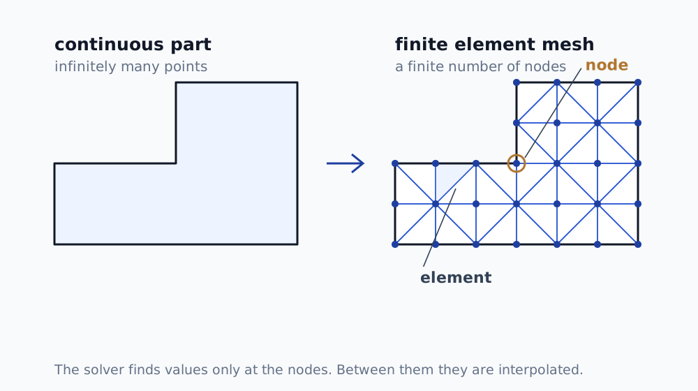
A real part has a continuous shape, so it has infinitely many points and a computer cannot solve it directly. The finite element method (FEM) divides it into elements and looks for values only at the nodes of the mesh. Everywhere between the nodes, values are filled in by interpolation.
What the solver really solves is the system
where is the stiffness matrix, the load and the unknown nodal displacements. There are no stresses here. Those are derived afterwards, from how fast the displacement changes between neighbouring nodes — that is, from the gradient.
One practical consequence follows: displacements are always more reliable than stresses. Differentiation makes accuracy worse. A model can give deflection with an error under one per cent and stresses with an error of tens of per cent at the same time. So when somebody defends an analysis by saying the deflection matches the measurement, they have proved nothing about the stresses.
Elements that cannot do bending
The second thing: the element type leaves a bigger mark on the result than the mesh density does.
A linear tetrahedron (TET4) has constant stress inside it. One number for the whole element. In bending, however, stress passes linearly through the thickness from tension into compression, which an element like that cannot represent even in principle. The structure comes out stiffer and the stresses lower than they really are.
Automatic meshing offers TET4 as the default because it is fast. But if the stresses are ones you are going to show somebody, switch to quadratic elements — TET10 or HEX20. The difference tends to be substantial.
The same applies to a single element through the wall thickness. Even with a good element type, that is too few. Three or more is a sensible starting point.
If a wavy mesh outline appears in your results that does not correspond to anything physical, the solver is fighting what is known as hourglassing — a zero-energy deformation mode of first-order elements with reduced integration. It is a warning, not a cosmetic defect: switch to full integration or to quadratic elements, or refine the mesh.
Where that red spot comes from
And the third thing, which answers the question from the introduction.
At a sharp re-entrant corner, the theory of elasticity predicts infinite stress. The same holds for a constraint applied at a single point and for a force introduced into a single node. It is not a fault of the mesh or of the software. It follows from the model having a perfectly sharp edge that a real part never has — a real part always has some radius, if only from the tool.
This is called a singularity, and stress in its vicinity behaves as
where is the distance from the corner tip. The exponent is what matters. While it is negative, stress grows without bound as you approach the corner. How strongly depends on the angle:
| Notch opening angle | Exponent |
|---|---|
| 0° (crack) | −0.50 |
| 90° | −0.46 |
| 120° | −0.38 |
| 180° (no notch) | 0 — no singularity |
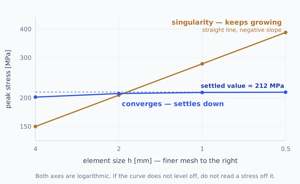
The smallest distance a mesh can resolve is the element size. That is why the peak stress at a singularity does not converge under mesh refinement, it grows — and it does so by a power law, that is, indefinitely.
That is why the maximum stress over the whole model is almost always an unusable figure, even though it is the first thing the software shows you. It is not the stress in the part. It is the stress at the place where the model lies.
What to do when that location matters for the assessment:
- model the real fillet radius that is actually there in the part,
- read the stress a little further away, outside the reach of the singularity,
- or use a procedure that accounts for the concentration — for welds, for example, structural stress extrapolated from distances prescribed by the relevant standard; for a crack, fracture mechanics.
What you must not do: keep refining the mesh until the number comes out nicely. At a singularity you are only making it bigger.
How to check that the mesh is fine enough
“I refined the mesh and nothing changed” is not evidence, because nobody knows by how much it did not change. Checking it is simple and costs a few hours of work.
Run the same problem on three meshes, halving the element size each time, and track one single value — for example the stress at the location you are assessing. There is more to pull out of those three numbers than it seems:
from math import log

def convergence(f1, f2, f3, r=2.0):
    """f1 = finest mesh, f3 = coarsest. r = element size refinement ratio."""
    # Order of convergence: how fast the result approaches the settled value.
    p = log(abs((f3 - f2) / (f2 - f1))) / log(r)
    # Estimate of the value at an infinitely fine mesh (Richardson extrapolation).
    settled = f1 + (f1 - f2) / (r**p - 1)
    # Error estimate of the finest result in per cent (the GCI, following Roache).
    error = 1.25 / (r**p - 1) * abs((f2 - f1) / f1) * 100
    return p, settled, error

# Stress [MPa] at element sizes of 1 / 2 / 4 mm.
p, settled, error = convergence(211.3, 209.1, 201.7)
print(f"order of convergence = {p:.2f}")
print(f"settled value        = {settled:.1f} MPa")
print(f"error estimate       = {error:.2f} %")

# order of convergence = 1.75
# settled value        = 212.2 MPa
# error estimate       = 0.55%
What to read from it:
- The order of convergence should come out positive, typically between 1 and 2. If it comes out negative, or the values jump around non-monotonically, you have no convergence and there is no point computing the rest. The most common cause is precisely a singularity.
- The error estimate is what belongs in the report, instead of a sentence about having refined the mesh. Half a per cent is a solid result; ten per cent means you need to go further.
This is not something I invented, it is standard practice — the ASME V&V 10 methodology for computational solid mechanics stands behind it (V&V 20 covers CFD), and in the literature it is known as the GCI (Grid Convergence Index).
The order of the numbers matters: f1 comes from the finest mesh. With the
order reversed, the exponent comes out negative, which is also the quickest way
to notice that you have made a mistake.
The fixed support that does not actually exist
Most genuinely bad results do not originate in the solver but in how the boundary conditions were set up. And you cannot see any of it in a colourful picture.
A perfect fixed support does not exist. A bolted joint has compliance. A weld has the stiffness of the plate around it. A mounting in a frame rotates slightly under load. When you simplify that in the analysis to “this face does not move”, the model comes out stiffer than reality and the stresses move somewhere other than where they really arise.
There is one small reprieve here, though. Saint-Venant’s principle says that the detail of exactly how you introduce a load stops mattering at a distance comparable with the size of the area through which you introduce it. If your location of interest is further away, the simplification does you no harm. If it is right at the fixing, it decides the entire result — and a force at a single node is, again, just a singularity.
When I review somebody else’s analysis, my first question is: which part of the assembly is missing here, and what did you replace it with? The answer says more about the quality of the model than any picture.
When a linear analysis stops being valid
Linear static analysis — what runs when you press the button — rests on three assumptions at once. One of them falling is enough for the result to be invalid.
The material stays in the elastic range. When von Mises stress locally exceeds the yield strength, a linear analysis over-predicts it, because it knows nothing about plastic redistribution. A value of 400 MPa in a material with a yield strength of 250 MPa says nothing about safety — that calls for an elastic-plastic analysis or a limit-load assessment.
Displacements are small compared with the dimensions. With large displacements, the geometry on which the analysis is being performed changes. Slender and thin-walled parts break this sooner than one would expect.
Contacts do not change during loading. Nothing separates and nothing seats. But as soon as the contact area changes, the problem is non-linear regardless of the material.
A non-linear analysis costs substantially more time, which is why it is not run casually. The decision whether to use one, however, has to be taken in advance, from the nature of the problem, not afterwards from what came out.
Be especially careful with loss of stability. A linear buckling analysis gives an upper bound, and for thin-walled shells the real critical load tends to be markedly lower, because manufacturing imperfections govern.
What an FEA report should contain
If you are buying in an analysis, the deliverable should not be a picture. For it to be defensible in front of a customer and repeatable in a year’s time when the part changes, the report should state:
- the CAD revision the analysis is based on, with its date,
- the element type and order, and the number of elements through the thickness at critical locations,
- the boundary conditions described in words, not just as a screenshot,
- the source of the material data,
- evidence of convergence, with an error estimate,
- the assessment criterion and where it comes from,
- a list of simplifications, including what was left out of the model and why.
Bonus: when you have to work through hundreds of variants
Full FEM is needlessly expensive for that. For the design phase, a simplified model can be trained on a small number of solutions; it then answers in milliseconds and also returns a measure of uncertainty. There is a demo you can click through and compare against an exact FEM solution on the page about FEA services.
The final analysis is still done with FEM. This is for searching, not for proof.
If you are working on a specific problem and cannot judge whether the result is sound, get in touch. Usually it can be settled from a few questions about the element type, the fixings, and what the convergence study says.
Frequently asked questions
- Why does stress in a sharp corner never converge?
- Because theory predicts infinite stress at a sharp re-entrant corner. The finer the mesh, the higher the number, and it never settles. This is not a software bug — it follows from the model having a sharp edge that the real part does not have. The real part has a fillet radius.
- Which mesh should I use when I need stresses?
- Quadratic elements: TET10 rather than TET4. A linear tetrahedron has constant stress inside it, so it cannot represent bending at all and will under-predict the result until you put many elements through the thickness. For stresses you intend to defend, TET4 is not worth it.
- How do I check that the mesh is fine enough?
- Run the same problem on three meshes, halving the element size each time, and track one single value. If it changes by a few per cent between the last two, you have converged. If it keeps climbing, you are watching a singularity.
- When is a linear static analysis not enough?
- When the material goes past yield, when displacements are large compared with the dimensions of the part, or when contacts change during loading. Any one of these is enough for the result to apply to a different problem from the one you set up.