In the article on buckling and loss of stability I wrote about a component that passes a strength check and fails anyway — because its capacity is governed by stiffness, not strength. Vibration is the other half of the same story. A component can be strong enough and stiff enough and still cause trouble, if something excites it at one of its natural frequencies. The displacement can then grow to large values; with no damping, theoretically without limit. It need not mean failure straight away — more often it first shows up as shaking and noise.
I had exactly such a case on my desk: a long slender duralumin tube, part of the control linkage of a machine, pinned at both ends. Two problems at once. The first was buckling — the bare tube did not reach the required critical load. The second was resonance: the first bending frequency of the tube lay dangerously close to the drive excitation at idle, and showed itself as an unpleasant rise in noise. This article, though, is about the second problem — and about the two tools used to diagnose it: modal and harmonic analysis. In the end a single measure solved both problems — a composite braid at mid-span of the tube; why that one, I show at the end of the article.
This article is also a signpost to the other articles in the series, which take the individual pieces further: reading a Campbell diagram, how to avoid resonance and multi-objective optimisation.
What a natural frequency and a mode shape are
Every structure has frequencies at which it starts to vibrate easily — a small excitation is enough and the displacement grows. These are its natural frequencies. Each one has a mode shape (a mode) belonging to it: the characteristic shape the structure takes up when excited at that frequency. A string has one half-wave in its first shape, two in the second, three in the third — and a beam or a tube is the same; a plate likewise, only in two directions.
Resonance occurs when the excitation hits a natural frequency. Energy then accumulates from cycle to cycle and only damping keeps the displacement in check. That is why a natural frequency is a quantity you need to know before the component goes into service with some periodic source — a drive, a gearbox, a pump.
What matters is what sets that frequency. For a simple vibrating system it is
where is stiffness and is mass. [1][2] The whole strategy can be read out of that formula: if I want the frequency higher, I add stiffness or take mass away; if I want it lower, the opposite. The strength of the material does not appear in it, just as it did not appear in Euler's formula for buckling.
Modal analysis: the map of resonances
Modal analysis is the computation of natural frequencies and mode shapes. In FEM it is an eigenvalue problem — the same mathematical form as buckling, only with a different second matrix. For undamped vibration you look for a non-trivial solution of the system
where is the stiffness matrix and the mass matrix. The condition for a non-trivial solution, , gives the natural angular frequencies (from which ) and the mode shapes belonging to them. [3][4]
The solver returns the mode shapes ordered by increasing frequency. A mode shape has no absolute size — it is a ratio of displacements between points, not millimetres. It says where the structure will move, not by how much; that second question is already a job for harmonic analysis.
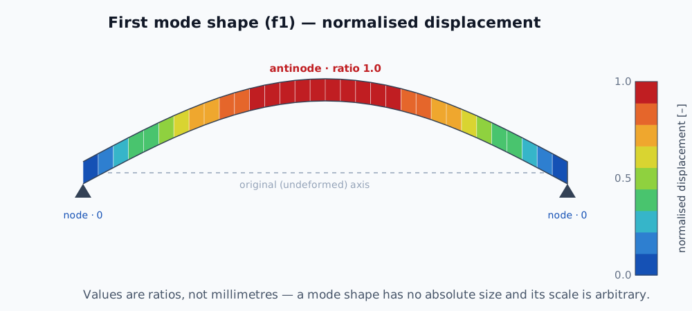
The first mode shape as a contour FE map (schematic). The colour is normalised displacement — zero at the nodes, unity at the antinode. Deliberately without millimetres: the solver gives only ratios of displacements between points and picks the scale of the shape itself. Absolute figures come only with harmonic analysis.
Why frequencies are computed on a prestressed structure
The stress state of a structure changes its stiffness. It is the same geometric stiffness that governs buckling: compression takes stiffness away, tension adds it. The source of the stress need not be an axial force — internal pressure in a thin-walled vessel, centrifugal force in a rotating blade or bolt preload all act the same way. When prestress is included in the modal problem, the stiffness matrix is corrected for it:
The consequence is easy to picture. In a strut a compressive force lowers the natural frequency — and as it approaches the critical buckling load, the first natural frequency goes to zero. Loss of stability can therefore be understood as “resonance at zero frequency” (in dynamics it is called divergence): the structure loses its stiffness in the first shape entirely. Tension, conversely, raises the frequency, because the component is being stiffened. [4][5]
For a pin-ended strut this relationship has a closed form, , where is the compressive axial force and the critical buckling load. As the first natural frequency goes exactly to zero — so in theory a large compressive force means failure (buckling) at zero frequency. [6]
That same dependence can be used the other way round: by measuring the frequency under increasing load (safely up to about 50 per cent of the critical load) and extrapolating the straight line of against force to zero frequency, the critical buckling load is obtained non-destructively. That is the essence of the vibration correlation technique (VCT). [7]
In tension the picture is different. The frequency rises in tension — elastically up to the yield strength, then only mildly — as far as the ultimate strength, and the fall to zero here does not happen gradually: at fracture the frequency drops to zero in a step. Both extremes of axial force therefore end at zero frequency, but differently: in compression falls continuously (buckling is a gradual loss of stiffness), in tension it is a discontinuous event (fracture).
That is why in a prestressed modal analysis every mode has three values: in compression (the lower frequency), unloaded (neutral) and in tension (higher). For this tube I assessed the neutral state for unloaded idling and the compression-to-tension range for operation, where the axial force varies in both directions. For the bare tube the operating compression of 1100 N is in fact above the critical load (~1067 N), so the compressive state is only worth computing with the braid in place.
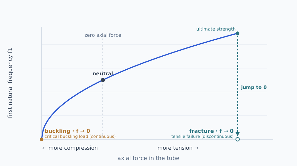
Axial force changes stiffness, and with it the natural frequency. In compression it falls continuously to zero at buckling; in tension it rises as far as the ultimate strength and at fracture drops to zero in a step. Both extremes end at zero frequency, but the compressive event is continuous (buckling) and the tensile one discontinuous (fracture).
The mode shapes of the bare tube
A bare tube with pinned–pinned ends has its first three bending shapes where we expect them — one, two and three half-waves of a sine along the length:
| Mode | Frequency | Shape | Symmetry |
|---|---|---|---|
| f1 | 18.04 Hz | 1st bending, 1 half-wave | symmetric |
| f3 | 71.96 Hz | 2nd bending, 2 half-waves | antisymmetric |
| f5 | 161.05 Hz | 3rd bending, 3 half-waves | symmetric |
The frequency ratio 18.04 : 71.96 : 161.05 ≈ 1 : 4 : 9 agrees with the theory of a pin-ended beam (, where is the number of half-waves) to within 1 per cent — which doubles as a check on the model.
The numbers 1, 3, 5 are not a typo. The tube has a circular section, so every bending shape exists in two mutually perpendicular planes at the same frequency — the modes come in pairs (f1 and f2, f3 and f4, …). For a planar problem the lower one out of each pair is enough, hence the odd numbers. The symmetry of a shape is not cosmetic: a few lines further down we will see what decides which mode can be excited at all.
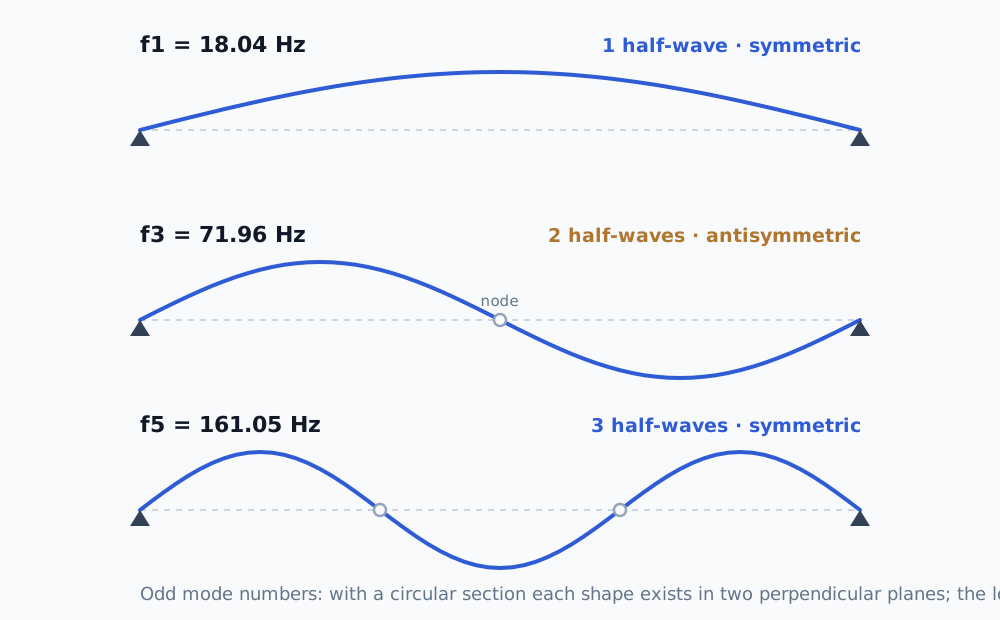
The first three bending shapes of a pin-ended tube. The symmetric shapes (1 and 3 half-waves) have an antinode at mid-span; the antisymmetric one (2 half-waves) has a node there. That symmetry decides which mode can be excited by which excitation.
Harmonic analysis: from frequencies to displacements
Modal analysis says where the resonances are. It does not say how much the component moves in them — because a mode shape has no size. That is what harmonic analysis is for: it computes the steady-state response of a structure to harmonic (sinusoidal) excitation across a whole range of frequencies. The result is a frequency response function (FRF) — a plot of displacement against excitation frequency, with a peak at every natural frequency that gets excited.
For this tube the excitation was the shaking of its mountings, not a force on the component itself — the drive shakes the whole assembly. That is what is known as base excitation. I computed it by mode superposition (MSUP), which assembles the response out of the mode shapes; it is cheap and accurate as long as enough modes above the band of interest are included (here at least up to about 300 Hz for a band up to 200 Hz). [5]
I applied the excitation as a unit gravitational acceleration (1 g). The result is then a “displacement per g”, and the real acceleration level is multiplied in later. I chose constant damping, , as an estimate for bare duralumin in its mountings (without a measurement).
I took the displacement as the maximum over the whole slender part, not at a single point — mid-span is a node of f3, and a probe there would not show it at all.
What came out of it
| Mode | Frequency | Displacement per 1 g | Ratio to f1 |
|---|---|---|---|
| f1 | 18.04 Hz | 98.3 mm | 100 % (reference) |
| f3 | 71.96 Hz | 3.18 mm | 3.2 % |
| f5 | 161.05 Hz | 0.44 mm | 0.45 % |
f1 and f5 come from the analysis with in-phase excitation, f3 from the anti-phase one (1 g at each support).
The first resonance vibrates with an order-of-magnitude larger displacement than the others — f3 is about thirty times milder and f5 more than two hundred times (see the table). For f5, which is excited by the same in-phase excitation as f1, two effects add up: a higher mode is stiffer and couples more weakly to uniform shaking of the supports. [8] The f3 figure comes from the anti-phase analysis, so its ratio to f1 only holds if the in-phase and anti-phase components of the excitation are equally strong. That is precisely why an FRF is drawn with a logarithmic vertical axis — on a linear one you would see only the first peak and the rest would merge into zero.
The plot has two curves, not one: each belongs to a different phase of the base excitation. The blue one (in phase) excites the symmetric shapes f1 and f5, the orange one (anti-phase) the antisymmetric f3. Why that is so is taken apart in the next section — here it is enough that no single curve shows all the resonances at once.
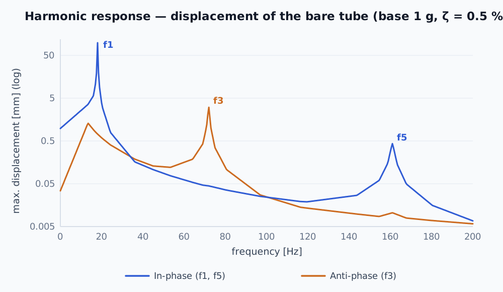
Two harmonic responses, each for a different phase of the base excitation: the blue one (in phase) excites the symmetric f1 and f5, the orange one (anti-phase) the antisymmetric f3. The position of a peak says whether the excitation reaches it; its height says how strongly.
Why the phase of the excitation decides which shapes come alive
The tube has alternately symmetric and antisymmetric shapes — and not every one of them can be excited by any excitation. What decides is the phase with which its two supports move.
- In phase (both supports alike, 0°/0°) the motion is pure translation of the whole assembly. It “displaces” the entire tube uniformly, so it excites only the symmetric shapes — f1 and f5. The antisymmetric f3 has a zero modal participation factor against such an excitation: one half of the tube would need to go up and the other down, but a uniform excitation pushes them the same way, so the contributions cancel. f3 does not come alive, even if its frequency lay exactly inside the excitation band.
- In anti-phase (supports opposed, 0°/180°) the motion is a rocking one. That excites the antisymmetric f3, while the symmetric f1 and f5 now cancel.
This holds exactly for a symmetric structure with identical mountings; any asymmetry partly restores the coupling.
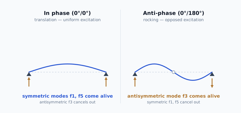
The phase of the base excitation decides the symmetry of the response. Translation (left) excites the symmetric shapes, rocking (right) the antisymmetric ones. That is why you need two analyses — a single analysis with one rigid base will never show the antisymmetric shape.
The practical consequence: for the full picture you need two analyses. Standard base excitation in a solver can usually handle only one rigid base (0°/0°), so antisymmetry has to be entered as a separate motion of each support with a phase shift. Anyone who runs only one analysis simply will not see the antisymmetric response and will believe that nothing excites that mode.
A relative comparison without absolute inputs
One question remains, and it troubles every problem of this kind: what is the real level of excitation and of damping? Without a measurement — an accelerometer on the mounting and a tap test [9] — I do not know them. And that is exactly why computing a unit excitation was worth doing.
Under a unit input the ratios between resonances are independent of the real level of excitation, and with the same damping on all modes, of the damping too. The height of a resonant peak is proportional to , so with a constant ζ it cancels in the ratio of two peaks.
That relationship has two assumptions: the damping is light () and the peaks are far enough apart for the height of each to be governed by a single mode. Here both are satisfied with a large margin. At the width of a peak (the half-power bandwidth, ) is only 0.18 Hz at f1 and 1.6 Hz at f5, while the neighbouring natural frequencies are tens of hertz away — the peaks therefore do not overlap and each belongs to one mode. [9] If the frequencies lay close together, or the damping were heavy, the peaks would merge and the ratio could not be cancelled down like this.
The result can therefore be stated as a ratio — the operating resonance vibrates with an order-of-magnitude smaller displacement than the one at idle — and that holds whatever figure the excitation finally turns out to be.
A known operating state, idling for instance, serves as the reference. The response is related to it instead of to an absolute “X millimetres”, which has nothing to stand on without a measurement. A relative statement — how much milder each resonance is than the one at idle — is verifiable even without absolute inputs.
Limits on its validity:
- It holds for displacement, not stress. Higher modes have greater curvature, so in fatigue they will be relatively worse than the ratio of displacements suggests.
- The real g differs between idling and operation. The ratio holds for the same input; absolute figures are filled in once a measurement is available.
- Multiples of 1 g / 2 g / 3 g are pointless in a linear analysis — displacement is directly proportional to the excitation, so one analysis and scaling are enough. They would only make sense with a non-linearity, for example clearance in the pin joints.
- Comparing f3 with f1 assumes equally strong in-phase and anti-phase components of the excitation. Their real ratio will only show up in a measurement at both supports.
Back to the component: one braid, two problems
The answer to both problems at once was a composite braid at mid-span of the tube — layers of carbon laid at an angle, with a glass separating layer against galvanic corrosion between the carbon and the aluminium. The braid does two things at the same time:
- it adds stiffness → it raises the critical buckling load and removes the first problem;
- it adds mass → it lowers the first natural frequency and moves it away from the drive excitation at idle.
Why does f1 fall rather than rise? At an angle of ±45° the carbon has a modulus of only about 9.3 GPa along the axis of the tube, so the braid adds relatively little bending stiffness but a noticeable amount of mass.
In a modal analysis these changes work against each other — and that is the whole core of the problem. For buckling I want high stiffness; for retuning the idle condition I want a lower frequency, which through the added mass works against higher stiffness. How far to run the braid and how many layers to lay up is not a single number but a region of compromise. There is a separate article on multi-objective optimisation about that.
Before any of that, though, you need to be able to read precisely where the resonances arise — that is what the Campbell diagram is for — and which of them are genuinely dangerous, because, as the small responses of f3 and f5 suggested, not every coincidence of a frequency with an excitation means trouble. That is the subject of the article How to avoid resonance.
References
- Rao, S. S. Mechanical Vibrations, Pearson.
- Den Hartog, J. P. Mechanical Vibrations, Dover Publications, 1985 (reprint of the 4th edition, McGraw-Hill, 1956).
- Thomson, W. T., Dahleh, M. D. Theory of Vibration with Applications, 5th edition, Prentice Hall, 1998.
- Cook, R. D., Malkus, D. S., Plesha, M. E., Witt, R. J. Concepts and Applications of Finite Element Analysis, 4th edition, Wiley, 2002 (prestressed modal analysis, geometric stiffness).
- Bathe, K.-J. Finite Element Procedures, Prentice Hall, 1996.
- Bokaian, A. Natural frequencies of beams under compressive axial loads, Journal of Sound and Vibration 126(1), 49–65 (1988), DOI 10.1016/0022-460X(88)90397-5. See also Blevins, R. D. Formulas for Natural Frequency and Mode Shape, Van Nostrand Reinhold, 1979.
- Arbelo, M. A. et al. Vibration Correlation Technique for the Estimation of Real Boundary Conditions and Buckling Load of Unstiffened Plates and Cylindrical Shells, Thin-Walled Structures 79, 119–128 (2014), DOI 10.1016/j.tws.2014.02.006; for struts classically Souza, M. A. et al. (1983). It builds on Southwell.
- Chopra, A. K. Dynamics of Structures: Theory and Applications to Earthquake Engineering, Prentice Hall (modal participation factor under base excitation).
- Ewins, D. J. Modal Testing: Theory, Practice and Application, 2nd edition, Research Studies Press, 2000.
Frequently asked questions
- What is the difference between modal and harmonic analysis?
- Modal analysis tells you where a structure has its natural frequencies and which mode shapes belong to them — that is, where resonance can arise. Harmonic analysis takes it from there and tells you how much the component really moves under a given excitation. Modal analysis is the map of resonances; harmonic analysis puts an amplitude against each of them.
- Why are natural frequencies computed on a prestressed structure?
- Because prestress changes stiffness. Tensile stress stiffens a structure and raises its frequencies; compressive stress softens it and lowers them — in a strut the first natural frequency goes to zero as the compressive force approaches the critical buckling load. The source of the stress need not be an axial force: internal pressure in a thin-walled vessel, centrifugal force in a rotating blade or bolt preload all act the same way. That is why in a problem like this every mode has a different value in compression, unloaded, and in tension.
- Why do higher modes vibrate with a smaller displacement than the first?
- The height of a resonant peak is proportional to Γ/(2ζω²) — the modal participation factor divided by the square of the natural angular frequency. A higher mode has a larger ω and, under uniform base excitation, a smaller Γ as well, because its alternating half-waves cancel each other in the integral; both terms push the displacement down. The exact power law depends on the structure and on the shape of the excitation — for this tube f5 came out more than two hundred times milder than f1. It holds for displacement, not for stress: higher modes have greater curvature and come out relatively worse in fatigue.
- Why does the phase of the base excitation decide which modes are excited?
- When both supports move in phase, the motion is pure translation and only symmetric shapes are excited. When they move in anti-phase, the motion is a rocking one and antisymmetric shapes are excited. A mode with the opposite symmetry to the excitation has a zero modal participation factor and never comes alive, even if its frequency falls exactly inside the excitation band. That is why you need two analyses.
- What use is unit excitation when I do not know the real acceleration?
- It gives a relative comparison without absolute inputs. Under unit excitation of 1 g the result is a displacement per g, and the ratios between resonances are independent of the real level of excitation — and, with the same damping on all modes, of the damping too. That is how you can show that the operating resonance vibrates with an order-of-magnitude smaller displacement than the one at idle, that is, than a known reference state, with absolute figures filled in once a measurement is available.