In another article I described how a non-linear analysis of a thin shell kept dying on me, and how I found that loss of stability was behind it rather than an error in the model. This article is a step back — to the theory that makes sense of it. Without that theory, buckling is just a number out of the solver; with it, you know what the number means and when you can believe it.
When equilibrium is stable
Picture a ball. In a hollow it is stable — nudge it and it returns. On top of a hill it is unstable — the slightest nudge sends it away. On a flat surface it is neutral — it stays wherever you put it. A structure behaves in exactly the same way, except that instead of the position of the ball we watch its deformed shape, and instead of gravity the load does the work.
Loss of stability is the point at which an originally stable equilibrium position stops being stable. The critical load is the value at which that happens. It is not the point where the material fails — it is the point where the structure moves into a different shape, even though the stress may still be far below the ultimate strength. That is precisely what makes buckling treacherous: a classical stress check does not catch it. [1]
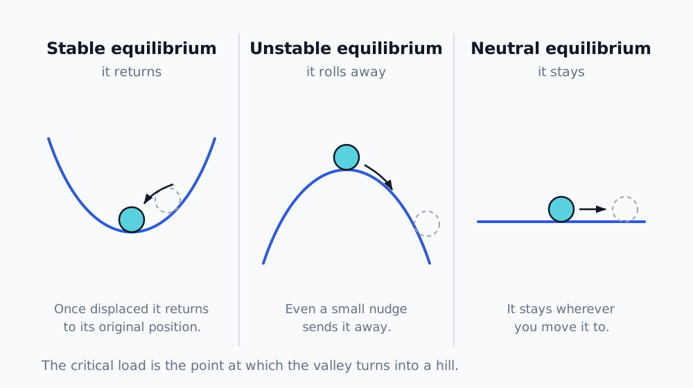
Stability of equilibrium: a ball in a hollow returns after being displaced, on a hill it escapes, on a plane it stays put. The critical load is the point where the hollow turns into a hill.
Euler: why buckling is governed by stiffness, not strength
The classical case is a strut in compression. Leonhard Euler showed that it buckles at the critical force
where is the modulus of elasticity, the second moment of area and the length. The key thing about this formula is what is not in it: the ultimate strength of the material. The critical buckling load depends on stiffness (), geometry (, ) and the end conditions — not on how strong the material is. [1]
That has a direct consequence, one I have also seen in practice: whether acrylic is brittle or ductile, the critical load for loss of stability does not change. The material governs what happens after stability is lost (whether it cracks, or bends and survives) and it governs the stresses — but the point of instability itself is driven by stiffness and shape. This is why a thin structure can be designed so that it passes the strength check and still buckles at a fraction of the design load.
Which end conditions the formula applies to — and what K is
The form above holds for a strut pinned at both ends (pinned–pinned): both ends can rotate freely but cannot move sideways. That is the reference, "basic Euler" case, and it buckles into a single half sine wave. [1]
Other end conditions are covered by the effective length factor . An effective (buckling) length is introduced and the formula generalises to
expresses what length the strut "sees" when it buckles, compared with the pin-ended case. A smaller = stiffer end restraint = a higher critical load. Careful: this has nothing to do with the stiffness matrix in the next section — it is only a historical coincidence of letters.
| End conditions | Theoretical K | Design K (AISC 360) | Effective length | Pcr vs pinned–pinned |
|---|---|---|---|---|
| pinned – pinned (basic Euler) | 1.0 | 1.0 | L | 1× |
| fixed – fixed | 0.5 | 0.65 | 0.5 L | 4× |
| fixed – pinned | 0.7 | 0.80 | 0.7 L | ≈ 2× |
| fixed – free end (cantilever) | 2.0 | 2.10 | 2 L | 0.25× |
There is a reason for the two columns. The theoretical values follow from the exact solution for perfect restraint (a perfect pin, a perfect fixity). The recommended design values (AISC 360, commentary, table C-A-7.1) are deliberately higher — a real connection is never infinitely stiff, so the calculation is made more conservative. [2]
And it all holds only under the assumptions that belong to Euler: an ideally straight, concentrically compressed, prismatic strut, linear elastic material below the proportional limit, small displacements up to the point of buckling, no imperfections — and only for sufficiently slender struts. Short, stocky ones fail plastically first and Euler would over-predict them; there you move to the buckling curves — in Europe those of EN 1993-1-1, cl. 6.3.1, which also cover imperfections and the inelastic range. [1][2]
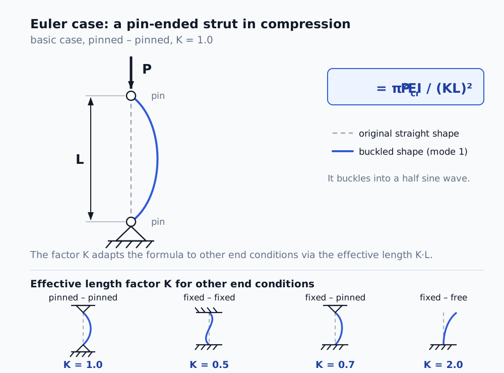
The basic Euler case (pinned–pinned, K = 1). The effective length factor K adapts the formula to other end conditions through the effective length KL.
Two mechanisms: bifurcation versus limit point
Not every loss of stability looks the same. [1][4]
Bifurcation buckling is the Euler case. A perfect strut sits on a straight equilibrium path — it compresses but stays straight. At the critical load a second, buckled equilibrium path appears and the structure "jumps" onto it. It is a branching of equilibrium — one path up to the critical point, two beyond it.
A limit point (snap-through) has no branching. The loading path rises smoothly, reaches a maximum and snaps over — the structure "snaps through" into a more remote shape. Typical of shallow arches and shells: a flat dome pressed from above suddenly snaps inwards at a certain point. On the force–displacement curve this shows up as a peak beyond which the force falls.
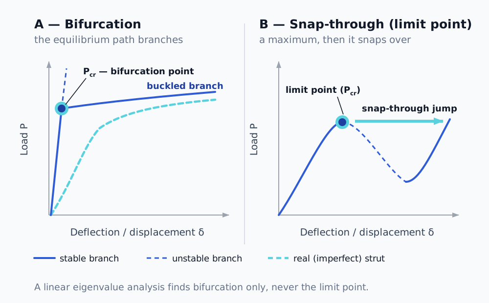
Two mechanisms of loss of stability. Bifurcation (left) branches the equilibrium path at the critical point; snap-through (right) reaches a maximum and snaps over. A linear eigenvalue analysis finds the first type only.
The difference is not academic. A linear eigenvalue analysis reliably finds bifurcation; it does not find a limit point — that has to be chased down non-linearly, because it is a large-displacement phenomenon. And a third dimension enters here: local versus global instability. Global instability flips the whole structure over (and is a genuine limit of load-carrying capacity). Local instability collapses only a region while the rest still carries — and the solver can die on it even though the structure as a whole is nowhere near collapsing. Telling these two apart is the single most important decision in practice.
Imperfection sensitivity: why reality never reaches Euler
Euler's formula applies to a perfect structure. A real one has deviations of shape, eccentricity of load, residual stresses — and those matter more than one would expect. A strut will take roughly 90% of the theoretical value. A thin shell in compression is another world: a cylinder loaded axially commonly carries only 20–30% of what linear theory predicts, and it is imperfections that govern that spread. This is why shell design works with knock-down factors — the theoretical value is an upper, optimistic estimate. [4][6]
The Southwell method: getting the critical force out of subcritical data
Tied to imperfections is an elegant tool that I used as an independent check on the critical load. The Southwell method estimates it without your having to push the structure all the way into buckling — it works with subcritical measurements only. [3]
Derivation (for a pin-ended strut)
Take a pin-ended strut with a small initial geometric imperfection in the shape of the first mode (a half sine wave) with amplitude at mid-span. Denote the load ratio .
Axial load amplifies the initial bow. The total mid-span deflection grows as
The additional deflection (over the initial, unloaded shape) is therefore
Dividing this equation by and rearranging drops out a linear relationship — the core of the whole method:
Which means: if you plot on the vertical axis against on the horizontal axis, you get a straight line whose
- slope , so the critical load is ,
- intercept on the axis , so the imperfection amplitude is .
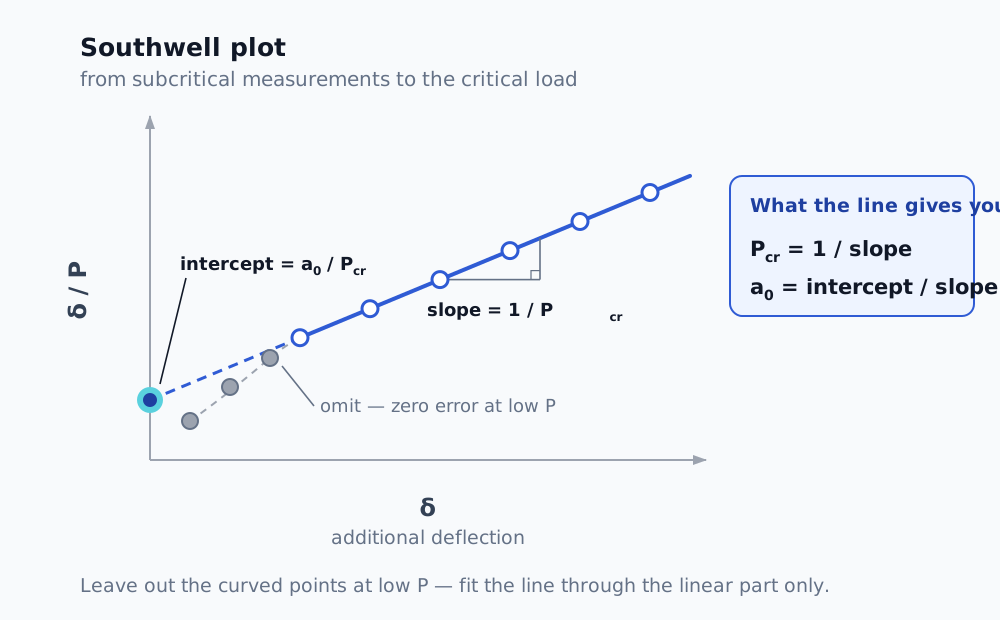
A line fitted through the subcritical points gives you two things at once: the reciprocal slope gives the critical load, the intercept on the vertical axis the amplitude of the initial imperfection. The curved points at low loads do not belong in the fit.
How to apply it in practice
- Load the strut in steps and, at several levels of in the subcritical range, measure the lateral deflection at mid-span (ideally the additional one, that is, relative to the unloaded shape).
- For each point work out the ratio .
- Plot the points and fit a straight line through them (linear regression).
- The critical load is the reciprocal of the slope. The intercept on the vertical axis gives the imperfection amplitude .
- Quality check: the points have to lie on a straight line. Curvature at low is usually an error in the zero of the deflection measurement — leave those first points out and fit the linear part only.
There is also a variant with the axes swapped — against — where the slope equals directly. The result is identical, you are only looking at the inverted line.
A note on the range of validity: the original Southwell method is derived for elastic bifurcation buckling of a prismatic strut. For plasticity, plates and shells there are extensions (Donnell, 1938, for example) which change which quantity is plotted against which. [3]
How buckling is computed in FEA — three levels
Linear (eigenvalue) buckling analysis. Mathematically, buckling is an eigenvalue problem. In the most common, textbook form it is written as
and a non-trivial solution exists only when the determinant of the matrix is zero — that is the characteristic equation , whose roots are the eigenvalues . For buckling the problem takes the generalised form
where is the elastic (classical) stiffness matrix and the geometric stiffness matrix, which depends on the state of stress in the structure. The condition for a non-trivial solution
gives the critical load factors and the buckling mode shapes that belong to them. The smallest positive is the critical load factor you are after — multiply by it and you have . It is fast, it gives an upper bound and the mode shapes, but it ignores imperfections, large displacements and non-linear material. That is why it over-predicts for shells, sometimes by a multiple. I treat it as diagnostics and a ceiling, not as a result. [5]
Non-linear statics (NLGEOM) with incremental loading. This captures the limit point, because it computes large displacements and changes the stiffness with the deformation. The trouble is that it freezes at the limit point — an implicit static scheme cannot get through a drop in force without help.
Arc-length (Riks) or quasi-static dynamics. This does get through the limit point. The arc-length method solves for load and displacement together, so it copes with the descending branch as well; a quasi-static transient lets the phenomenon run dynamically, the way it happens in reality. The rule that quasi-statics holds as long as the kinetic energy stays small compared with the strain energy belongs here too.
The sequence is clear: eigenvalue buckling for quick diagnostics and a ceiling, non-linear statics to locate the limit point, arc-length or dynamics to get through it and onto the post-buckling path.
Where the theory meets practice
This is exactly the chain I went through in the thin-shell case mentioned above. Eigenvalue buckling gave me factors below 1 and said "watch out, there is buckling here" — but as a shell upper bound I did not believe it as a result. Southwell, from subcritical data, confirmed the critical load independently. And the difference between local and global instability decided whether the convergence failure meant collapse or merely the limit of a static method.
Buckling theory is not just a chapter from a textbook. It is the framework that turns a series of solver warnings into an intelligible physical story — and it protects you from two opposite mistakes: believing the optimistic linear number, or declaring collapse where only the method has failed.
What that looked like on a specific job is in the article Non-linear FEA not converging.
References
- Timoshenko, S. P., Gere, J. M. Theory of Elastic Stability, 2nd edition, McGraw-Hill, 1961.
- EN 1993-1-1, cl. 6.3.1 (buckling curves, imperfection factors, buckling length) — the governing code for European design. Supplementary: AISC 360, Specification for Structural Steel Buildings, commentary, table C-A-7.1 (theoretical and recommended design values of the effective length factor).
- Southwell, R. V. On the Analysis of Experimental Observations in Problems of Elastic Stability, Proc. Roy. Soc. London, Series A, 135, 601–616 (1932). DOI 10.1098/rspa.1932.0055. Extension: Donnell, L. H., 1938.
- Bažant, Z. P., Cedolin, L. Stability of Structures: Elastic, Inelastic, Fracture and Damage Theories, Oxford University Press.
- Cook, R. D., Malkus, D. S., Plesha, M. E., Witt, R. J. Concepts and Applications of Finite Element Analysis, 4th edition, Wiley, 2002; Bathe, K.-J. Finite Element Procedures, Prentice Hall, 1996.
- NASA SP-8007, Buckling of Thin-Walled Circular Cylinders (knock-down factors for shells).
Frequently asked questions
- Does the critical buckling load depend on the strength of the material?
- No. Euler's formula contains the modulus of elasticity, the second moment of area, the length and the end conditions — the ultimate strength is not in it. The material governs what happens after stability is lost, and it governs the stresses, but the point of instability itself is driven by stiffness and shape.
- What is the difference between bifurcation and a limit point?
- At a bifurcation the equilibrium path branches at the critical point — a second, buckled position appears. A limit point (snap-through) does not branch: the loading path rises smoothly, reaches a maximum and snaps over. A linear eigenvalue analysis reliably finds bifurcation only.
- Why does linear buckling over-predict for shells?
- Because it assumes perfect geometry and ignores imperfections, large displacements and non-linear material. Thin-walled shells are extraordinarily sensitive to imperfections: an axially compressed cylinder commonly carries only 20 to 30 per cent of the linear prediction. That is why design works with knock-down factors.
- What is the effective length factor K for?
- It converts other end conditions to the basic pin-ended case through the effective length KL. A smaller K means stiffer end restraint and a higher critical load. The theoretical values hold for perfect restraint. EN 1993-1-1 works with the buckling length L_cr and the buckling curves; the American AISC quotes design K values that are deliberately higher, because a real connection is not infinitely stiff.
- What is the Southwell method?
- A procedure that estimates the critical load from subcritical measurements, without having to push the structure all the way into buckling. You plot the ratio of additional deflection to load against the additional deflection; the points lie on a straight line whose reciprocal slope is the critical load.